Leaning pandas. Data manipulation and visualization. (COVID-19 in - Scotland statistics)

Let's do a little bit of pandas. Pandas is (or are? :) extremely popular. Let's just dive in.
First of all, using pandas is the easiest way to open an Excel file. Just one line of code. Let's take, for example, this file -
Weekly deaths by location of death, age group, sex and cause, 2020 and 2021
(10 March 2021)
weekly-deaths-by-location-age-sex.xlsx
Taken from official the site:
https://www.nrscotland.gov.uk/.../related-statistics
import pandas as pd
data = pd.read_excel ('https://www.nrscotland.gov.uk/files//statistics/covid19/weekly-deaths-by-location-age-sex.xlsx',
sheet_name='Data',
skiprows=4,
skipfooter=2,
usecols='A:F',
header=None,
names=['week','location','sex','age','cause','deaths']
)
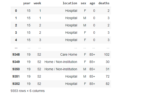
data
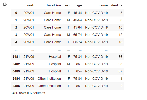
First of all, we can read the file directly from the Internet. The few parameters we used are self-explaining: we need to skip the first four rows, two last rows also of no interest. We also need to specify column headers, as in the original file, they somehow occupy both third and fourth rows and pandas is not able to detect them correctly. There are a lot of data, we'll try to use most of them later. But the first task will be to get simple totals by week. In SQL this would be achieved by using group by:
select sum(deaths) from data group by week
What is the equivalent in pandas?
import numpy as np
data.groupby('week').agg({'deaths': np.sum})
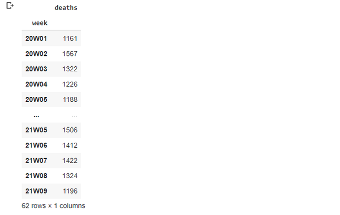
group by became groupby() method. A bit messy with sum: firstly, we had to import numpy as np, secondly, we had to use an additional function - agg(). The good news, with agg() we can use much more statistical function than any flavour of SQL would allow. np.median is probably the most noticeable example - there is no simple way to get median with SQL. And with agg() we can use our own functions as well.
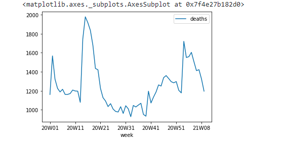
Let's plot a graph immediately!
data.groupby('week').agg({'deaths': np.sum}).plot()
Let's make it a bit bigger and add a title:
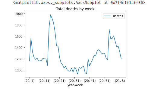
data.groupby('week').agg({'deaths': np.sum}).plot(figsize=(24,10),title='Total deaths by week')
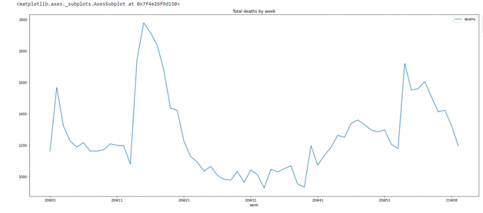
figsize is measured in inches, according to documentation. 24 x 10 seems to be fine for my screen.
Ok, we have a nice big chart with totals for the years 2020-2021. Let's add data for previous years, they just happened to be on the same web page:
Weekly deaths by location of death, age group and sex, 2015 to 2019
weekly-deaths-by-location-age-group-sex-15-19.xlsx
Web page:
https://www.nrscotland.gov.uk/.../related-statistics
data_1519 = pd.read_excel ('https://www.nrscotland.gov.uk/files//statistics/covid19/weekly-deaths-by-location-age-group-sex-15-19.xlsx',
sheet_name='Data',
skiprows=4,
skipfooter=2,
usecols='A:F',
header=None,
names=['year','week','location','sex','age','deaths'])
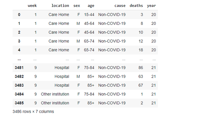
data_1519
The structure of the data is almost the same. There is no 'cause' column. Let's just add it:
data_1519['cause'] = 'Pre-COVID-19'
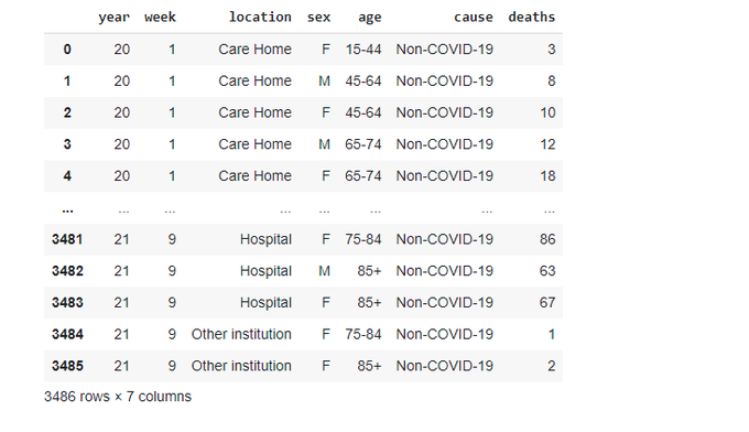
Let's rearrange the colums to make the DataFrame closer to our first data:
neworder =['year','week','location','sex','age','cause','deaths']
data_1519 = data_1519.reindex(columns=neworder)
data_1519
Now we need to do something with 'week' column of the first table. Let's split it into year and week to match the second table:
data_2021 = data # let's keep original DataFrame as is and work with a copy from now on
data_2021['year'] = data_2021.week.str.slice(0,2).astype(int)
data_2021['week'] = data_2021.week.str.slice(3,5).astype(int)
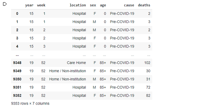
data_2021
And rearrage columns to match
neworder =['year','week','location','sex','age','cause','deaths']
data_2021 = data_2021.reindex(columns=neworder)
data_2021
We have to update our groupby function to reflect this change:
data_2021.groupby(['year','week']).agg({'deaths': np.sum}).plot(title='Total deaths by week')
Let's plot the 15/19 data the same way:
data_1519.groupby(['year','week']).agg({'deaths': np.sum}).plot(title='Total deaths by week')
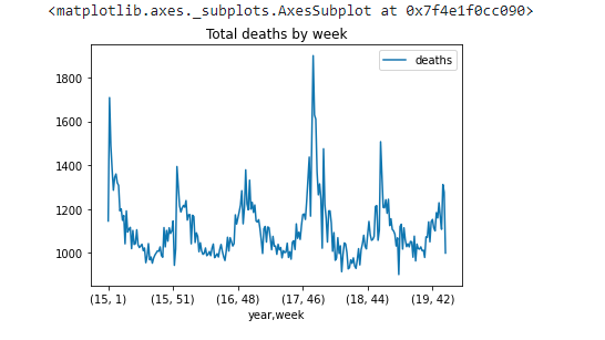
Apparently this is not what we wanted. Let's find an easy way forward.
I think it would make sense to save our groupby'd data in a new DataFrame and play with saved totals:
totals_1519 = data_1519.groupby(['year','week']).agg({'deaths': np.sum})
totals_1519['deaths_15'] = None
totals_1519['deaths_16'] = None
totals_1519['deaths_17'] = None
totals_1519['deaths_18'] = None
totals_1519['deaths_19'] = None

totals_1519
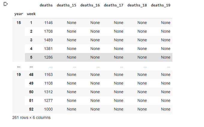
totals_1519.shape

(261,6)
What I wanted to do: create columns death_xx for each year, None by default, and then copy actual values only for a given year, leaving Nones in the columns for other years. And I couldn't accomplish this before I have realized that the DataFrame structure is somewhat different from what I expected - it has 6 columns (deaths, deaths_15, deaths_16, deaths_17, deaths_18, deaths_19) and one Multiindex (year, week) (I think Multiindex corresponds to a familiar Composite index in SQL). And the index isn't counted as columns, so we need to re-structure the DataFrame, using the following function:
totals_1519.reset_index(inplace=True)
totals_1519
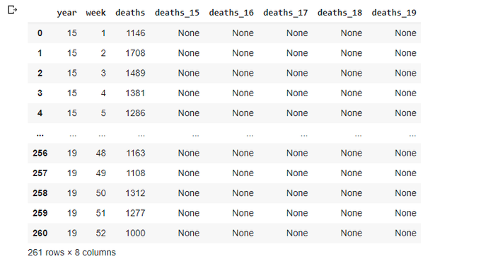
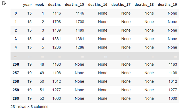
Let's populate deaths_xx columns as we wanted:
totals_1519.loc[totals_1519['year']==15,'deaths_15']=totals_1519['deaths']
totals_1519.loc[totals_1519['year']==16,'deaths_16']=totals_1519['deaths']
totals_1519.loc[totals_1519['year']==17,'deaths_17']=totals_1519['deaths']
totals_1519.loc[totals_1519['year']==18,'deaths_18']=totals_1519['deaths']
totals_1519.loc[totals_1519['year']==19,'deaths_19']=totals_1519['deaths']
totals_1519
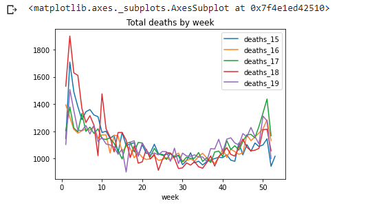
Now we can plot all 6 lines in a single graph:
totals_1519.plot(x='week',y=['deaths_15','deaths_16','deaths_17','deaths_18','deaths_19'],title='Total deaths by week')
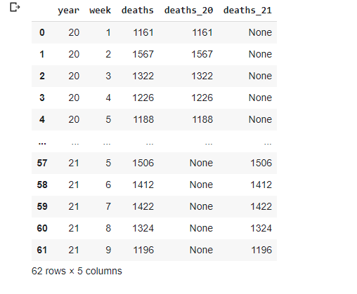
Let's do the same with the 20/21 data:
totals_2021 = data_2021.groupby(['year','week']).agg({'deaths': np.sum})
totals_2021['deaths_20'] = None
totals_2021['deaths_21'] = None
totals_2021.reset_index(inplace=True)
totals_2021.loc[totals_2021['year']==20,'deaths_20']=totals_2021['deaths']
totals_2021.loc[totals_2021['year']==21,'deaths_21']=totals_2021['deaths']
totals_2021
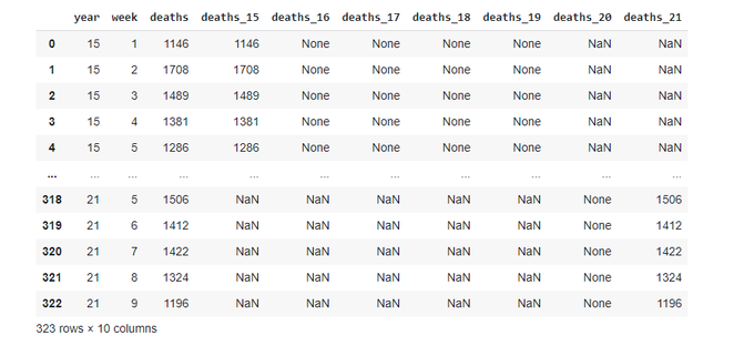
Now we are ready to combine two DataFrames into a final totals DataFrame. Two things to notice:
- pandas puts NaN, non None, in empty cells. Doesn't affect us in this case
- it is really difficult to predict which operations are performed in place and which return the new DataFrame...
totals = totals_1519
totals=totals.append(totals_2021,ignore_index=True)
totals
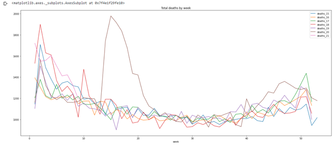
Let's plot the final totals:
totals.plot(x='week',y=['deaths_15','deaths_16','deaths_17','deaths_18','deaths_19','deaths_20','deaths_21'],title='Total deaths by week',figsize=(24,10))
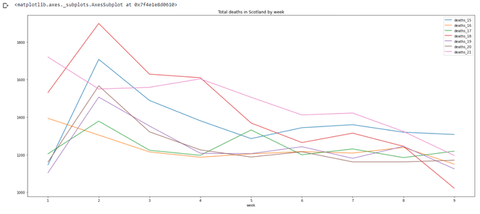
And to finish today's exercises let's concentrate on the first 9 weeks of the years:
totals[totals['week']<=9].plot(x='week',y=['deaths_15','deaths_16','deaths_17','deaths_18','deaths_19','deaths_20','deaths_21'],title='Total deaths in Scotland by week',figsize=(24,10))
The code for this article can be found on gist.github:
https://gist.github.com/vallka/ec6ac989aef1f1e26c5f282e84040984
and on Google Colab:
https://colab.research.google.com/drive/1Dh1aCNx_GD8cAWauJ4eP-yWqPOpH5SLC?usp=sharing
To be continued...